Quickstart
Installation
Install pqp using pip
pip install pqp
Usage
To characterize a causal effect, we need to specify three things:
Causal Assumptions: a graph representing the causal structural relationships between variables
Parametric Assumptions: a parametric model of the joint distribution of the data
Causal Estimand: an algebraic expression representing the causal effect of interest
Setup
To get started, we will spoof some data to run our analysis on.
import pandas as pd

df = pd.DataFrame({
    "x": [0, 0, 0, 1, 1, 0],
    "z": [0, 1, 0, 1, 1, 0],
    "y": [0, 1, 0, 1, 1, 0],
})
We can use the make_vars function to create a list of variables.
from pqp.symbols import make_vars
x, y, z = make_vars("xyz")
Note that the names of these variables match the column names in the data frame.
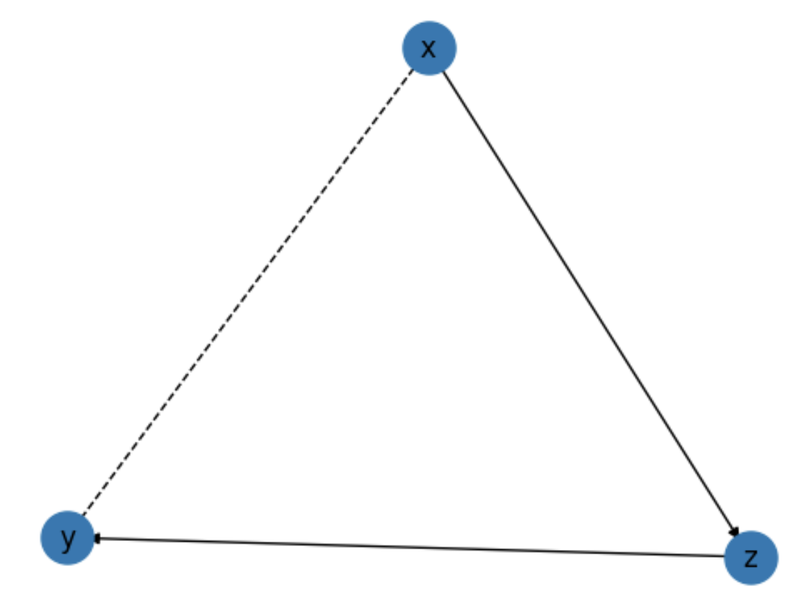
Causal Assumptions
We can then assemble these variables into a causal diagram using the Graph class. Here we will
build the famous front-door model.
Infix operators are used to construct causal relationships. The <= operator is used to
indicate causal influence from right to left, while the & operator is used to indicate
confounding.
from pqp.identification import Graph
g = Graph([
    x & y,
    z <= x,
    y <= z,
])
We can use the .draw() method to visualize the causal diagram.
g.draw()
Parametric Assumptions
For the purposes of this article, we will assume that the data is drawn from a multinomial
distribution. We can use the MultinomialEstimator class to specify the parametric assumptions.
from pqp.estimation import MultinomialEstimator
estimator = MultinomialEstimator(df, prior=1)
The prior argument specifies the prior strength of the model. The default is
zero, in which case the model fits through maximum likelihood. We are using a nonzero
value here because if you don’t specify a prior, the model will not always give positive
probability estimates to events, which can cause problems when estimating causal effects.
If you don’t specify a prior, don’t worry though. If the estimator runs into a problem, it will throw an exception and tell you what to do.
Causal Estimand
For this example, we will estimate the average treatment effect of x on y. First,
we need to define the treatment and control conditions.
treatment_condition = [x.val == 1]
control_condition = [x.val == 0]
Then, we can use the ATE class to define the causal estimand.
from pqp.identification import ATE
causal_estimand = ATE(y, treatment_condition, control_condition)

#inspect the expression
causal_estimand.expression().display()

Identification and Estimation
Now, we can first use the causal assumptions to identify the causal estimand, and then we can use the parametric assumptions to estimate the causal effect.
To identify the causal relationships in the causal diagram, we can use the .identify() method.
For example, to identify the causal relationship between x and y, we can use the following:
estimand = g.identify(causal_estimand).identified_estimand
estimand.display()
We can then use the .estimate() method to estimate the causal effect.
effect = estimator.estimate(estimand)
effect
# => EstimationResult(value=0.4433808167141502)
Interpretability and Robustness
One of the most important features of pqp is its ability to provide human-interpretable explanations of the workings of the code. Many of the routines make very specific assumptions about the structure of the data or the effects of interest. It’s important for users to understand these assumptions so they can understand the potential limitations of an analysis.
The currency of pqp is the Result class. Any calculations that draw conclusions from the data will return instances of this class. This class tracks the transformations and assumptions made by the algorithms. As Results are assembled into successively more complex analyses of the data, pqp builds a dependency graph which tracks how different Result instances relate to each other and allows the user access to a list of steps executed in an analysis and the assumptions made.
To access the list of steps, we can use the .explain() and explain_all() methods, which detail the current result only or all results in the dependency graph, respectively.
effect.explain_all()
Output:
Data Processing
Assume: x is on BinaryDomain()
Assume: z is on BinaryDomain()
Assume: y is on BinaryDomain()
Identification
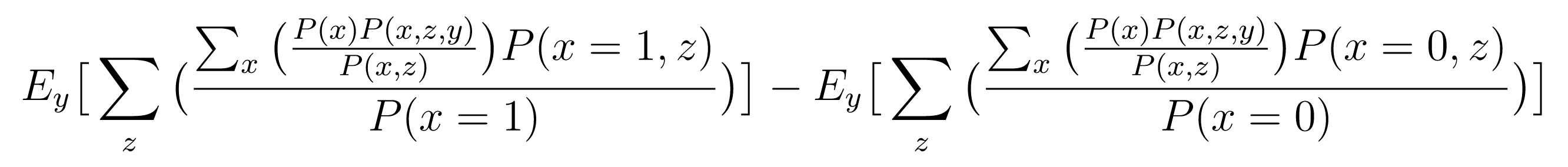
We will identify the average treatment effect using IDC.
Assume: Noncontradictory evidence
Assume: Acyclicity
Assume: Positivty
IDC
Input:
P(y| do(x))
Output:
Σ_(z) [ [Σ_(x) [ [P(x) * P(x, z, y) / P(x, z)] ] * P(x, z) / P(x)] ]
Derived: identified_estimand = E_(y) [ Σ_(z) [ [Σ_(x) [ [P(x) * P(x, z, y) / P(x, z)] ] * P(x = 1, z) / P(x = 1)] ] ] - E_(y) [ Σ_(z) [ [Σ_(x) [ [P(x) * P(x, z, y) / P(x, z)] ] * P(x = 0, z) / P(x = 0)] ] ]
Fit MultinomialEstimator
Assume: Multinomial likelihood
Assume: Dirichlet prior
Estimation
Performing brute force estimation using a multinomial likelihood and dirichlet prior.
Derived: value = 0.4433808167141502